How to Read Text File in Spark
Information
Has it occurred to yous that she might not accept been a reliable source of information?
— Jon Snowfall
With the noesis caused in previous chapters, you are now equipped to start doing analysis and modeling at scale! So far, however, we haven't really explained much about how to read data into Spark. Nosotros've explored how to use copy_to() to upload modest datasets or functions like spark_read_csv() or spark_write_csv() without explaining in item how and why.
And so, y'all are well-nigh to learn how to read and write data using Spark. And, while this is of import on its own, this affiliate will also introduce y'all to the data lake—a repository of data stored in its natural or raw format that provides various benefits over existing storage architectures. For case, you lot can easily integrate data from external systems without transforming information technology into a common format and without assuming those sources are as reliable as your internal information sources.
In addition, we will too discuss how to extend Spark'southward capabilities to work with data not accessible out of the box and brand several recommendations focused on improving performance for reading and writing data. Reading large datasets often requires you to fine-tune your Spark cluster configuration, but that's the topic of Affiliate 9.
Overview
In Affiliate 1, you learned that beyond big information and big compute, you can besides employ Spark to ameliorate velocity, variety, and veracity in data tasks. While you can employ the learnings of this affiliate for any task requiring loading and storing data, it is specially interesting to nowadays this affiliate in the context of dealing with a multifariousness of information sources. To understand why, we should first take a quick detour to examine how information is currently candy in many organizations.
For several years, it's been a common practice to store large datasets in a relational database, a arrangement outset proposed in 1970 by Edgar F. Codd.21 You can think of a database as a collection of tables that are related to ane another, where each table is carefully designed to hold specific information types and relationships to other tables. Most relational database systems use Structured Query Language (SQL) for querying and maintaining the database. Databases are still widely used today, with good reason: they shop data reliably and consistently; in fact, your bank probably stores account balances in a database and that'south a practiced practise.
Yet, databases have also been used to shop information from other applications and systems. For instance, your bank might also store data produced by other banks, such as incoming checks. To accomplish this, the external data needs to be extracted from the external system, transformed into something that fits the current database, and finally exist loaded into it. This is known as Extract, Transform, and Load (ETL), a general procedure for copying data from one or more sources into a destination arrangement that represents the information differently from the source. The ETL process became popular in the 1970s.
Aside from databases, data is oftentimes besides loaded into a data warehouse, a system used for reporting and data analysis. The information is usually stored and indexed in a format that increases information analysis speed but that is often not suitable for modeling or running custom distributed code. The challenge is that irresolute databases and data warehouses is commonly a long and delicate process, since information needs to be reindexed and the data from multiple data sources needs to be carefully transformed into single tables that are shared across data sources.
Instead of trying to transform all data sources into a mutual format, you can embrace this diversity of data sources in a data lake, a organisation or repository of data stored in its natural format (see Figure viii.1). Since data lakes brand data available in its original format, there is no demand to carefully transform it in advance; anyone can employ information technology for analysis, which adds significant flexibility over ETL. Y'all then can use Spark to unify information processing from information lakes, databases, and information warehouses through a single interface that is scalable across all of them. Some organizations also use Spark to supercede their existing ETL process; however, this falls in the realm of data technology, which is well beyond the scope of this volume. We illustrate this with dotted lines in Figure 8.1.
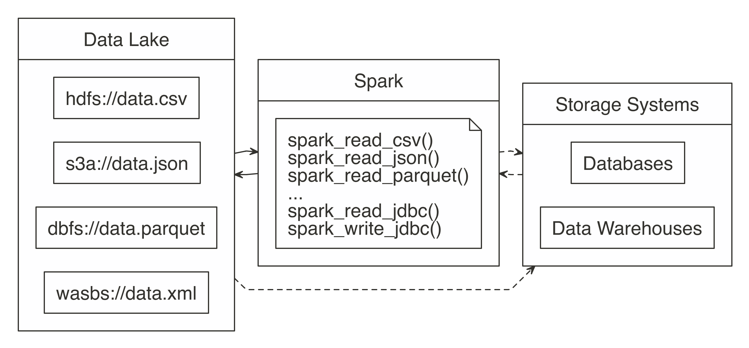
Effigy 8.one: Spark processing raw information from a data lakes, databases, and data warehouses
In order to support a broad diverseness of data source, Spark needs to be able to read and write data in several different file formats (CSV, JSON, Parquet, etc), admission them while stored in several file systems (HDFS, S3, DBFS, etc) and, potentially, interoperate with other storage systems (databases, data warehouses, etc). We will go to all of that; but showtime, we will starting time past presenting how to read, write and copy data using Spark.
Reading Data
To support a broad diversity of data sources, Spark needs to exist able to read and write data in several unlike file formats (CSV, JSON, Parquet, and others), and admission them while stored in several file systems (HDFS, S3, DBFS, and more) and, potentially, interoperate with other storage systems (databases, data warehouses, etc.). We will get to all of that, just first, we will start by presenting how to read, write, and copy data using Spark.
Paths
If you are new to Spark, it is highly recommended to review this section earlier you commencement working with large datasets. Nosotros volition introduce several techniques that improve the speed and efficiency of reading information. Each subsection presents specific means to have advantage of how Spark reads files, such as the ability to treat entire folders as datasets as well equally being able to describe them to read datasets faster in Spark.
letters <- data.frame(x = letters, y = i : length(letters)) dir.create("data-csv") write.csv(letters[1 : 3, ], "data-csv/letters1.csv", row.names = Simulated) write.csv(letters[1 : three, ], "data-csv/letters2.csv", row.names = FALSE) do.call("rbind", lapply(dir("data-csv", full.names = True), read.csv)) x y 1 a 1 2 b 2 3 c iii four a ane v b 2 half dozen c 3 In Spark, there is the notion of a folder as a dataset. Instead of enumerating each file, simply laissez passer the path containing all the files. Spark assumes that every file in that binder is part of the same dataset. This implies that the target folder should be used only for information purposes. This is especially important since storage systems like HDFS store files across multiple machines, only, conceptually, they are stored in the same folder; when Spark reads the files from this folder, it'south really executing distributed code to read each file within each machine—no data is transferred between machines when distributed files are read:
# Source: spark<datacsv> [?? x 2] x y <chr> <int> i a 1 ii b 2 3 c 3 4 d 4 v due east five 6 a ane 7 b 2 8 c 3 9 d 4 10 e 5 The "binder as a tabular array" idea is found in other open source technologies as well. Under the hood, Hive tables work the aforementioned way. When you query a Hive table, the mapping is done over multiple files within the same folder. The binder'due south proper noun commonly matches the proper noun of the tabular array visible to the user.
Next, we will present a technique that allows Spark to read files faster likewise equally to reduce read failures by describing the construction of a dataset in advance.
Schema
When reading data, Spark is able to make up one's mind the information source'southward column names and column types, too known equally the schema. Withal, guessing the schema comes at a cost; Spark needs to do an initial pass on the data to approximate what it is. For a large dataset, this tin can add a significant amount of time to the data ingestion process, which tin can get costly even for medium-size datasets. For files that are read over and over once again, the boosted read time accumulates over time.
To avoid this, Spark allows y'all to provide a cavalcade definition by providing a columns argument to draw your dataset. You can create this schema by sampling a small portion of the original file yourself:
ten y "factor" "integer" Or, you can set the column specification to a vector containing the column types explicitly. The vector's values are named to match the field names:
10 y "character" "numeric" The accepted variable types are: integer, grapheme, logical, double, numeric, factor, Date, and POSIXct.
So, when reading using spark_read_csv(), you lot can laissez passer spec_with_r to the columns argument to match the names and types of the original file. This helps to ameliorate performance since Spark will not need to make up one's mind the column types.
# Source: spark<datacsv> [?? ten 2] x y <chr> <int> 1 a one 2 b two 3 c 3 four a 1 5 b 2 6 c 3 The following instance shows how to gear up the field type to something different. However, the new field type needs to be a compatible type in the original dataset. For example, you cannot set a character field to numeric. If you lot utilize an incompatible blazon, the file read will fail with an error. Additionally, the following instance also changes the names of the original fields:
# Source: spark<datacsv> [?? 10 2] my_letter my_number <chr> <chr> ane a 1 2 b ii 3 c 3 iv a ane five b 2 half-dozen c iii In Spark, malformed entries can crusade errors during reading, particularly for non-character fields. To prevent such errors, we can use a file specification that imports them as characters and and so use dplyr to coerce the field into the desired blazon.
This subsection reviewed how we tin read files faster and with fewer failures, which lets us start our analysis more chop-chop. Some other style to advance our analysis is by loading less information into Spark memory, which we examine in the adjacent section.
Memory
Past default, when using Spark with R, when you read data, it is copied into Spark's distributed retentiveness, making data analysis and other operations very fast. There are cases, such every bit when the information is too big, for which loading all the data might non exist practical or even necessary. For those cases, Spark can just "map" the files without copying data into retentiveness.
The mapping creates a sort of virtual tabular array in Spark. The implication is that when a query runs against that table, Spark needs to read the information from the files at that fourth dimension. Whatever consecutive reads afterward that will do the aforementioned. In consequence, Spark becomes a pass-through for the data. The reward of this method is that at that place is virtually no up-forepart time cost to "reading" the file; the mapping is very fast. The downside is that running queries that actually excerpt data will have longer.
This is controlled past the retention argument of the read functions. Setting information technology to FALSE prevents the data copy (the default is TRUE):
In that location are good utilize cases for this method, one of which is when not all columns of a tabular array are needed. For example, take a very large file that contains many columns. Assuming this is not the first time you lot collaborate with this data, you lot would know what columns are needed for the assay. When you know which columns you need, the files can be read using memory = Faux, so the needed columns can exist selected with dplyr. The resulting dplyr variable can so exist cached into memory, using the compute() function. This volition brand Spark query the file(southward), pull the selected fields, and copy but that data into retentivity. The result is an in-memory tabular array that took comparatively less time to ingest:
The next department covers a brusque technique to arrive easier to comport the original field names of imported data.
Columns
Spark ane.half-dozen required that column names exist sanitized, so R does that past default. At that place might be cases when you would similar to keep the original names intact, or when working with Spark version two.0 or above. To exercise that, prepare the sparklyr.sanitize.column.names option to Simulated:
# Source: table<iris> [?? ten 5] # Database: spark_connection Sepal.Length Sepal.Width Petal.Length Petal.Width Species <dbl> <dbl> <dbl> <dbl> <chr> ane 5.1 3.5 one.four 0.ii setosa two iv.9 3 1.4 0.2 setosa 3 4.7 3.2 1.3 0.2 setosa 4 4.six 3.1 1.5 0.2 setosa five 5 3.6 one.four 0.2 setosa 6 5.iv 3.9 one.7 0.4 setosa 7 4.half-dozen 3.four 1.4 0.3 setosa 8 v 3.four 1.v 0.ii setosa 9 4.4 2.nine 1.4 0.2 setosa 10 4.nine iii.1 ane.5 0.ane setosa # ... with more rows With this review of how to read data into Spark, we motility on to expect at how we tin can write data from our Spark session.
Writing Information
Some projects require that new data generated in Spark be written back to a remote source. For example, the information could exist new predicted values returned by a Spark model. The task processes the mass generation of predictions, but then the predictions need to be stored. This section focuses on how y'all should use Spark for moving the information from Spark into an external destination.
Many new users start by downloading Spark data into R, and and so upload it to a target, every bit illustrated in Figure 8.two. It works for smaller datasets, just it becomes inefficient for larger ones. The data typically grows in size to the signal that it is no longer feasible for R to be the middle point.
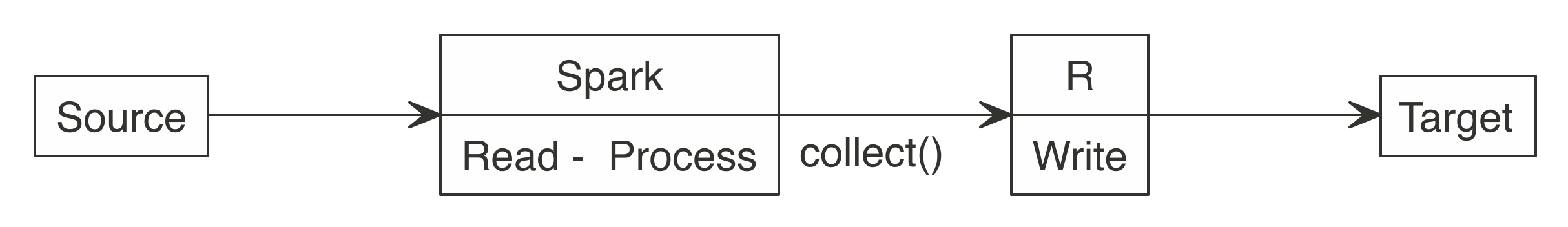
Figure eight.2: Incorrect use of Spark when writing big datasets
All efforts should be fabricated to have Spark connect to the target location. This fashion, reading, processing, and writing happens within the aforementioned Spark session.
Equally Figure 8.3 shows, a meliorate approach is to use Spark to read, procedure, and write to the target. This approach is able to scale equally big as the Spark cluster allows, and prevents R from becoming a choke point.
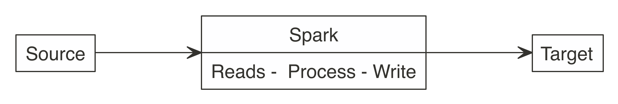
FIGURE 8.iii: Correct use of Spark when writing large datasets
Consider the following scenario: a Spark job just processed predictions for a big dataset, resulting in a considerable amount of predictions. Choosing a method to write results will depend on the technology infrastructure y'all are working on. More specifically, information technology will depend on Spark and the target running, or not, in the same cluster.
Back to our scenario, we have a large dataset in Spark that needs to be saved. When Spark and the target are in the aforementioned cluster, copying the results is non a problem; the information transfer is between RAM and disk of the same cluster or efficiently shuffled through a high-bandwidth connection.
But what to practice if the target is not within the Spark cluster? In that location are 2 options, and choosing ane will depend on the size of the data and network speed:
- Spark transfer
- In this case, Spark connects to the remote target location and copies the new data. If this is done within the same datacenter, or cloud provider, the information transfer could be fast enough to take Spark write the data direct.
- External transfer and otherwise
- Spark can write the results to deejay and transfers them via a third-party application. Spark writes the results as files and and then a carve up chore copies the files over. In the target location, you lot would use a divide process to transfer the data into the target location.
It is all-time to recognize that Spark, R, and whatsoever other engineering science are tools. No tool can do everything, nor should be expected to. Adjacent nosotros will describe how to re-create data into Spark or collect large datasets that don't fit in-retentivity, this can be used to transfer information beyond clusters, or help initialize your distributed datasets.
Re-create
Previous chapters used copy_to() every bit a handy helper to copy data into Spark; however, you can use copy_to() only to transfer in-memory datasets that are already loaded in memory. These datasets tend to be much smaller than the kind of datasets y'all would want to re-create into Spark.
For instance, suppose that we have a 3 GB dataset generated every bit follows:
If we had simply 2 GB of memory in the driver node, we would non exist able to load this three GB file into memory using copy_to(). Instead, when using the HDFS every bit storage in your cluster, you lot can use the hadoop command-line tool to re-create files from disk into Spark from the final as follows. Detect that the following code works only in clusters using HDFS, not in local environments.
Yous and so tin can read the uploaded file, as described in the File Formats section; for text files, you would run:
# Source: spark<largefile> [?? x 1] line <chr> 1 0.0982531064914565 -0.577567317599452 -1.66433938237253 -0.20095089489… 2 -i.08322304504007 1.05962389624635 i.1852771207729 -0.230934710049462 … iii -0.398079835552421 0.293643382374479 0.727994248743204 -i.571547990532… iv 0.418899768227183 0.534037617828835 0.921680317620166 -1.6623094393911… v -0.204409401553028 -0.0376212693728992 -1.13012269711811 0.56149527218… half-dozen 1.41192628218417 -0.580413572014808 0.727722566256326 0.5746066486689 … 7 -0.313975036262443 -0.0166426329807508 -0.188906975208319 -0.986203251… 8 -0.571574679637623 0.513472254005066 0.139050812059352 -0.822738334753… 9 1.39983023148955 -1.08723592838627 1.02517804413913 -0.412680186313667… 10 0.6318328148434 -1.08741784644221 -0.550575696474202 0.971967251067794… # … with more rows collect() has a similar limitation in that it can collect only datasets that fit your driver retentivity; even so, if you had to extract a large dataset from Spark through the commuter node, you could employ specialized tools provided by the distributed storage. For HDFS, you would run the following:
Alternatively, you can too collect datasets that don't fit in memory by providing a callback to collect(). A callback is just an R function that will exist called over each Spark partition. You and so can write this dataset to deejay or push to other clusters over the network.
You could employ the following code to collect 3 GB even if the driver node collecting this dataset had less than 3 GB of retentivity. That said, as Affiliate iii explains, you should avoid collecting large datasets into a unmarried machine since this creates a meaning operation bottleneck. For conciseness, nosotros volition collect only the start 1000000 rows; feel free to remove head(x^6) if you lot have a few minutes to spare:
Make sure you clean up these large files and empty your recycle bin as well:
In most cases, data will already be stored in the cluster, and then you should not need to worry about copying big datasets; instead, y'all tin usually focus on reading and writing dissimilar file formats, which we describe adjacent.
File Formats
Out of the box, Spark is able to interact with several file formats, like CSV, JSON, LIBSVM, ORC, and Parquet. Tabular array eight.1 maps the file format to the function y'all should use to read and write information in Spark.
| Format | Read | Write |
|---|---|---|
| Comma separated values (CSV) | spark_read_csv() | spark_write_csv() |
| JavaScript Object Annotation (JSON) | spark_read_json() | spark_write_json() |
| Library for Support Vector Machines (LIBSVM) | spark_read_libsvm() | spark_write_libsvm() |
| Optimized Row Columnar (ORC) | spark_read_orc() | spark_write_orc() |
| Apache Parquet | spark_read_parquet() | spark_write_parquet() |
| Text | spark_read_text() | spark_write_text() |
The following sections will draw special considerations particular to each file format likewise as some of the strengths and weaknesses of some popular file formats, starting with the well-known CSV file format.
CSV
The CSV format might be the most common file blazon in use today. It is defined by a text file separated by a given character, usually a comma. It should be pretty straightforward to read CSV files; however, it's worth mentioning a couple techniques that can help you procedure CSVs that are not fully compliant with a well-formed CSV file. Spark offers the following modes for addressing parsing issues:
- Permissive
- Inserts Cypher values for missing tokens
- Drop Malformed
- Drops lines that are malformed
- Fail Fast
- Aborts if it encounters any malformed line
You tin use these in sparklyr past passing them inside the options argument. The following example creates a file with a broken entry. It then shows how information technology can exist read into Spark:
# Source: spark<bad3> [?? x 1] foo <int> 1 1 2 ii three three Spark provides an consequence tracking column, which was hidden by default. To enable it, add together _corrupt_record to the columns listing. You can combine this with the use of the PERMISSIVE way. All rows will be imported, invalid entries volition receive an NA, and the issue volition exist tracked in the _corrupt_record cavalcade:
# Source: spark<bad2> [?? ten 2] foo `_corrupt_record` <int> <chr> one i NA 2 2 NA 3 three NA iv NA broken Reading and storing data as CSVs is quite common and supported beyond most systems. For tabular datasets, information technology is still a popular choice, simply for datasets containing nested structures and nontabular data, JSON is unremarkably preferred.
JSON
JSON is a file format originally derived from JavaScript that has grown to be language-independent and very popular due to its flexibility and ubiquitous support. Reading and writing JSON files is quite straightforward:
# Source: spark<data> [?? x ii] a b <dbl> <listing> ane i <listing [ii]> However, when you deal with a dataset containing nested fields similar the one from this instance, it is worth pointing out how to extract nested fields. One approach is to employ a JSON path, which is a domain-specific syntax commonly used to extract and query JSON files. You can use a combination of get_json_object() and to_json() to specify the JSON path you are interested in. To extract f1 y'all would run the post-obit transformation:
# Source: spark<?> [?? x 3] a b z <dbl> <list> <chr> 1 i <list [two]> 2 Another approach is to install sparkly.nested from CRAN with install.packages("sparklyr.nested") and and so unnest nested data with sdf_unnest():
# Source: spark<?> [?? x 3] a f1 f3 <dbl> <dbl> <dbl> 1 1 two 3 While JSON and CSVs are quite elementary to use and versatile, they are not optimized for performance; however, other formats similar ORC, AVRO, and Parquet are.
Parquet
Apache Parquet, Apache ORC, and Apache AVRO are all file formats designed with performance in mind. Parquet and ORC store data in columnar format, while AVRO is row-based. All of them are binary file formats, which reduces storage infinite and improves performance. This comes at the cost of making them a bit more difficult to read by external systems and libraries; still, this is usually not an issue when used as intermediate data storage within Spark.
To illustrate this, Effigy 8.4 plots the result of running a ane-one thousand thousand-row write-speed benchmark using the demote package; feel free to use your own benchmarks over meaningful datasets when deciding which format all-time fits your needs:
numeric <- copy_to(sc, data.frame(nums = runif(ten ^ 6))) bench:: mark( CSV = spark_write_csv(numeric, "information.csv", fashion = "overwrite"), JSON = spark_write_json(numeric, "data.json", mode = "overwrite"), Parquet = spark_write_parquet(numeric, "data.parquet", mode = "overwrite"), ORC = spark_write_parquet(numeric, "information.orc", mode = "overwrite"), iterations = twenty ) %>% ggplot2:: autoplot() 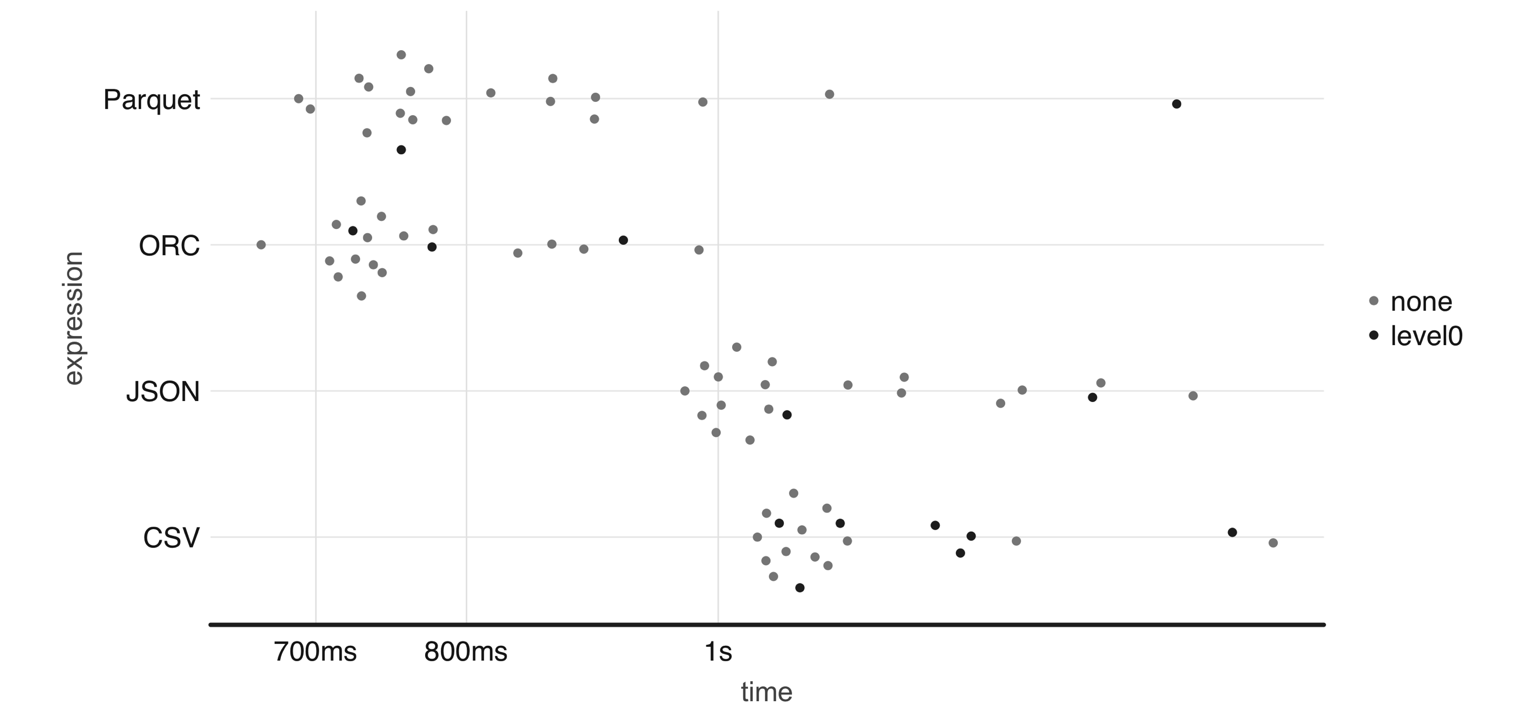
Effigy eight.4: One-million-rows write benchmark between CSV, JSON, Parquet, and ORC
From now on, be sure to disconnect from Spark whenever we nowadays a new spark_connect() command:
This concludes the introduction to some of the out-of-the-box supported file formats, we will present next how to deal with formats that crave external packages and customization.
Others
Spark is a very flexible computing platform. Information technology tin add functionality past using extension programs, chosen packages. Yous can admission a new source type or file system past using the appropriate parcel.
Packages need to be loaded into Spark at connection time. To load the bundle, Spark needs its location, which could be within the cluster, in a file share, or the net.
In sparklyr, the package location is passed to spark_connect(). All packages should be listed in the sparklyr.connect.packages entry of the connection configuration.
It is possible to admission data source types that we didn't previously list. Loading the appropriate default packet for Spark is the kickoff of two steps The second step is to actually read or write the data. The spark_read_source() and spark_write_source() functions do that. They are generic functions that tin use the libraries imported by a default package.
For instance, we can read XML files as follows:
# Source: spark<data> [?? x ane] text <chr> 1 Hullo Globe which you lot can also write back to XML with ease, as follows:
In add-on, there are a few extensions developed by the R community to load additional file formats, such as sparklyr.nested to aid with nested data, spark.sas7bdat to read data from SAS, sparkavro to read data in AVRO format, and sparkwarc to read WARC files, which use extensibility mechanisms introduced in Chapter ten. Chapter 11 presents techniques to use R packages to load boosted file formats, and Chapter 13 presents techniques to use Java libraries to complement this further. Only first, allow'due south explore how to retrieve and store files from several unlike file systems.
File Systems
Spark defaults to the file organization on which information technology is currently running. In a YARN managed cluster, the default file organization volition be HDFS. An example path of /home/user/file.csv will exist read from the cluster'south HDFS folders, non the Linux folders. The operating system's file system will be accessed for other deployments, such as Standalone, and sparklyr's local.
The file arrangement protocol tin be changed when reading or writing. You do this via the path statement of the sparklyr role. For example, a total path of _file://home/user/file.csv_ forces the use of the local operating arrangement's file system.
At that place are many other file arrangement protocols, such equally _dbfs://_ for Databricks' file arrangement, _s3a://_ for Amazon'south S3 service, _wasb://_ for Microsoft Azure storage, and _gs://_ for Google storage.
Spark does not provide support for all them straight; instead, they are configured equally needed. For example, accessing the "s3a" protocol requires calculation a package to the sparklyr.connect.packages configuration setting, while connecting and specifying advisable credentials might require using the AWS_ACCESS_KEY_ID and AWS_SECRET_ACCESS_KEY environment variables.
Accessing other file protocols requires loading different packages, although, in some cases, the vendor providing the Spark surround might load the package for yous. Please refer to your vendor's documentation to find out whether that is the case.
Storage Systems
A data lake and Spark usually go hand-in-paw, with optional access to storage systems like databases and data warehouses. Presenting all the different storage systems with appropriate examples would be quite time-consuming, so instead we present some of the commonly used storage systems.
As a start, Apache Hive is a data warehouse software that facilitates reading, writing, and managing large datasets residing in distributed storage using SQL. In fact, Spark has components from Hive built directly into its sources. It is very common to take installations of Spark or Hive side-past-side, so we will start past presenting Hive, followed by Cassandra, and then close by looking at JDBC connections.
Hive
In YARN managed clusters, Spark provides a deeper integration with Apache Hive. Hive tables are easily accessible after opening a Spark connection.
You tin access a Hive table's information using DBI by referencing the table in a SQL argument:
Another style to reference a table is with dplyr using the tbl() part, which retrieves a reference to the table:
It is important to reiterate that no data is imported into R; the tbl() part only creates a reference. You then can pipe more than dplyr verbs following the tbl() control:
Hive table references assume a default database source. Often, the needed table is in a dissimilar database within the metastore. To admission it using SQL, prefix the database proper name to the table. Separate them using a flow, as demonstrated hither:
In dplyr, the in_schema() function tin be used. The part is used inside the tbl() call:
You can also use the tbl_change_db() function to ready the current session'south default database. Whatsoever subsequent phone call via DBI or dplyr will use the selected name equally the default database:
The following examples require boosted Spark packages and databases which might be difficult to follow unless you happen to have a JDBC driver or Cassandra database attainable to y'all.
Next, we explore a less structured storage organization, frequently referred to as a NoSQL database.
Cassandra
Apache Cassandra is a complimentary and open source, distributed, wide-column shop, NoSQL database management system designed to handle large amounts of data beyond many article servers. While there are many other database systems beyond Cassandra, taking a quick look at how Cassandra can be used from Spark will give you insight into how to make use of other database and storage systems similar Solr, Redshift, Delta Lake, and others.
The post-obit example lawmaking shows how to utilize the datastax:spark-cassandra-connector package to read from Cassandra. The key is to apply the org.apache.spark.sql.cassandra library equally the source statement. It provides the mapping Spark tin can use to brand sense of the data source. Unless you take a Cassandra database, skip executing the following statement:
I of the nigh useful features of Spark when dealing with external databases and data warehouses is that Spark tin can button down ciphering to the database, a feature known as pushdown predicates. In a nutshell, pushdown predicates improve functioning by request remote databases smart questions. When you execute a query that contains the filter(age > 20) expression confronting a remote table referenced through spark_read_source() and non loaded in retention, rather than bringing the unabridged table into Spark, it will be passed to the remote database and simply a subset of the remote table is retrieved.
While it is platonic to find Spark packages that back up the remote storage organization, there will be times when a bundle is non available and you demand to consider vendor JDBC drivers.
JDBC
When a Spark packet is not available to provide connectivity, you can consider a JDBC connexion. JDBC is an interface for the programming linguistic communication Java, which defines how a client can access a database.
It is quite piece of cake to connect to a remote database with spark_read_jdbc(), and spark_write_jdbc(); as long as you have access to the appropriate JDBC driver, which at times is little and other times is quite an take a chance. To go along this unproblematic, we can briefly consider how a connection to a remote MySQL database could be accomplished.
First, you lot would demand to download the appropriate JDBC driver from MySQL'southward developer portal and specify this boosted commuter as a sparklyr.shell.commuter-class-path connection option. Since JDBC drivers are Java-based, the lawmaking is contained within a JAR (Java ARchive) file. Equally soon every bit you lot're connected to Spark with the advisable commuter, yous can use the jdbc:// protocol to access particular drivers and databases. Unless you are willing to download and configure MySQL on your own, skip executing the following statement:
If you are a customer of particular database vendors, making utilise of the vendor-provided resources is usually the best place to start looking for appropriate drivers.
Recap
This chapter expanded on how and why you should utilise Spark to connect and procedure a diversity of information sources through a new data storage model known every bit information lakes—a storage pattern that provides more than flexibility than standard ETL processes by enabling y'all to use raw datasets with, potentially, more data to enrich information analysis and modeling.
We too presented best practices for reading, writing, and copying data into and from Spark. We then returned to exploring the components of a data lake: file formats and file systems, with the one-time representing how data is stored, and the latter where the information is stored. You then learned how to tackle file formats and storage systems that crave additional Spark packages, reviewed some of the performance trade-offs across file formats, and learned the concepts required to make employ of storage systems (databases and warehouses) in Spark.
While reading and writing datasets should come naturally to you, you might nonetheless hit resource restrictions while reading and writing large datasets. To handle these situations, Chapter 9 shows you how Spark manages tasks and data across multiple machines, which in turn allows you to farther meliorate the performance of your analysis and modeling tasks.
lerouxtiledgets78.blogspot.com
Source: https://therinspark.com/data.html
0 Response to "How to Read Text File in Spark"
Post a Comment